Next: Kepler's Equation
Up: master
Previous: The General two Body
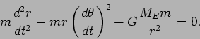
In this section we will prove that the solutions to the equation
of motion
are conic sections in general, and ellipses in
particular. For the sake of simplicity, we consider only
the simplified version for an earth orbiting satellite
(13). This equation gives  as a function of the
time
as a function of the
time  . From the previous section we know that the motion is
restricted to a plane. To continue we introduce polar coordinates
in this plane and write:
. From the previous section we know that the motion is
restricted to a plane. To continue we introduce polar coordinates
in this plane and write:
and hence
where
 is a unit vector perpendicular to
  , which
forms a right hand system together with .
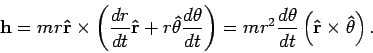
Using this we can rewrite the angular momentum as
, which
forms a right hand system together with .
Using this we can rewrite the angular momentum as
In particular, we have
where  is the area swept over by . The conservation of
angular momentum therefore directly implies Kepler's second law.
is the area swept over by . The conservation of
angular momentum therefore directly implies Kepler's second law.
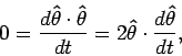
To continue observe that
and hence
 is perpendicular to
itself
and therefore
parallel to . It turns out that
is perpendicular to
itself
and therefore
parallel to . It turns out that
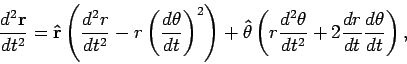
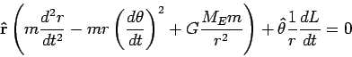
Combining all these properties we can write:
and the entire equation of motion becomes
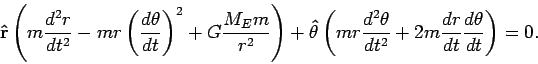
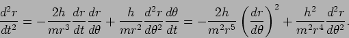
Using the expression for  above we get
Since the angular momentum is conserved
 we get
 |
(16) |
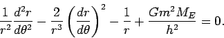
We can eliminate  by using
 . Doing this reduces the
equation of motion to a single non-linear second order ODE.
Observe that we started out with a system of three second order
non-linear ODE.
. Doing this reduces the
equation of motion to a single non-linear second order ODE.
Observe that we started out with a system of three second order
non-linear ODE.
What follows is a number of little tricks to simplify (16)
even further. First observe that
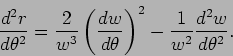
Differentiating this again with respect to we get
Plugging this into (16) we get after some algebra
 |
(17) |
All this did so far is change the independent variable from to
. (16) was a non-linear second order equation and as such difficult to solve.. To continue we make a change of dependent variable,
namely let
Then
and
We observe that this introduces another non-linear term of the form
However, after substituting this we see that this new nonlinear
term cancels with the existing nonlinear term and we get
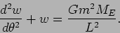 |
(18) |
This new equation is now a linear second order equation with
constant coefficients, the best of all possible worlds. This
equation is easy to solve and its solutions are of the form
 |
(19) |
where the constants and  depend on the initial
conditions.
After re-introducing
depend on the initial
conditions.
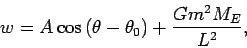
After re-introducing  we get:
 |
(20) |
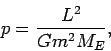
where
and
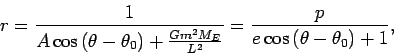
(20) is of course the well known equation of an ellipse
in polar coordinates with eccentricity  and focus at the
origin. We have thus established Kepler's first law, namely that
the orbits are elliptical.
and focus at the
origin. We have thus established Kepler's first law, namely that
the orbits are elliptical.
Next: Kepler's Equation
Up: master
Previous: The General two Body
Werner Horn
2006-06-06